Using and Testing Tensorflow Models in the Browser with AI Squared

By Ian Sotnek and Jacob Renn @ AI Squared

Running neural networks in the browser is a challenge! Between the lack of a Python environment and being constrained by the computing power of your local device getting models to run in the first place is hard enough. You don’t want to just run a model in the browser for its own sake though, you should be able to visualize the model results in real-time to assess the performance of the model and get real value from it. Let me show you how that could work with a model that you want to use in the browser.

Age prediction based on images of faces is a timely topic — just a few weeks ago, Instagram announced that machine learning-based age prediction is a new feature offered to users of their platform. Say you create a similar model, a model that classifies the decade of age of a person based on an image of their face, and then want to try it out on images that are available online: how would you experiment with the model you’ve created to see if it’s accurate enough to use in your production system? AI Squared was created to help with this kind of problem in mind! In this tutorial, we’ll walk you through how to train a model on the UTKFace dataset, then deploy that model to the AI Squared browser extension, where you can see the model running over images on web pages and give some feedback on whether the model is working as intended.

In the following parts of this blog we’ll create a Keras model, wrap that model in an AI Squared-compatible .air file, and then use the AI Squared extension to use the model to classify images in the browser. A Python notebook with all of the code in one place can be accessed in our GitHub.

With that, let’s dive in!

Part 1: Create the Model

1.1 Importing the required packages

This step imports some standard libraries in addition to the aisquared package.

1.2 Data Preparation

Here we set some important parameters for data preparation and augmentation to assist with training. Additionally, we create a function to load the data into a generator.

*Note — we used Databricks as our development environment so the dataset is stored in the Databricks file system, but you can point to any location on disk or in the cloud where you have the dataset stored.

1.3 Model Creation & Training

Here we create the model that will be trained. This model consists of two individual models in sequence. The first model performs data preprocessing and augmentation, including a rescaling of pixel values to [0, 1], random horizontal flips of input images, and random rotation of images. The second model contains the decision logic, containing multiple convolutional blocks which are then fed into a fully connected architecture for classification.

1.4 Evaluate the model

Here we evaluate the model on validation data.

Part 2: Create the .air file

Now that the model itself has been created and saved, we can create the .air file that can be used to integrate the model into the browser workflow. The configuration of the .air file includes steps to determine data harvesting, data preprocessing, the analytic or model that is to be run on the data, result postprocessing and rendering, as well as how users can input feedback into the model. If you have any questions at this stage, I recommend consulting the aisquared documentation site to get more detail about how you can configure a model to run in the browser.

2.1 Configure data harvesting

The aisquared package supports a handful of ways to gather input data from webpages or webapps. Here we are using the ImageHarvester class, which grabs all available images and passes them to the analytic defined in the analytic step.

2.2 Configure preprocessing steps

Some models, including the model created in part 1, expect input images to be resized and/or normalized. This step defines how all of the images gathered from the content of the webpage will be resized and normalized so that the model can process them accurately.

2.3 Identify the model that you want to use

In this step, you can point to the model that you want to use in the browser. In this case, we’re using the model you created in Step 1 and will be running it locally. However, this method also supports running models that have been deplyed to remote resources (e.g. Sagemaker) as well.

2.4 Configure postprocessing steps

When your model makes a classification, it is outputting some floating point or integer value, which might not be very informative when viewing your model results in the browser. In this step, we take the output of the model and apply a label map to it, so that what ends up rendered in the webpage is useful information.

2.5 Configure rendering of model outputs

Now that your model has made a classification and you’ve determined how that classification maps to a human-readable label, you get to define how those results are displayed on the webpage. We’re relying on the default values for image bounding boxes and label sizes, but you can change that easily with the information in the documentation.

2.6 Configure feedback widgets

Recall that you want to see how well your model is performing in the wild. Just looking at the model results on a webpage and noting instances of misclassification is a great first step, but AI Squared supports feedback widgets that let you create and log feedback about the model’s performance that you can download from the extension for further analysis. Here is how to create a basic feedback widget in aisquared:

2.7 Create and compile the configuration object

Now that all the steps have been defined, you can combine them using the ModelConfiguration object to pull them all together into a single configuration object that is ready to be compiled.

Once the configuration object is created, the .compile() method aggregates and stores the configuration as well as a converted version of the model itself into the .air package. It is important to note in this case that the model itself is stored in this file, meaning that when someone runs this file in the extension, the entire analytic workflow happens locally — no need to deploy the model to a remote resource (although we support that too). For details about the aisquared package, please see the documentation page.

Notice that a new .air file has been created in your working directory.

Part 3: Using the .air File

Now for the fun part — using your model in the browser!

The next step is to visit the Chrome store and install the free AI Squared Extension.

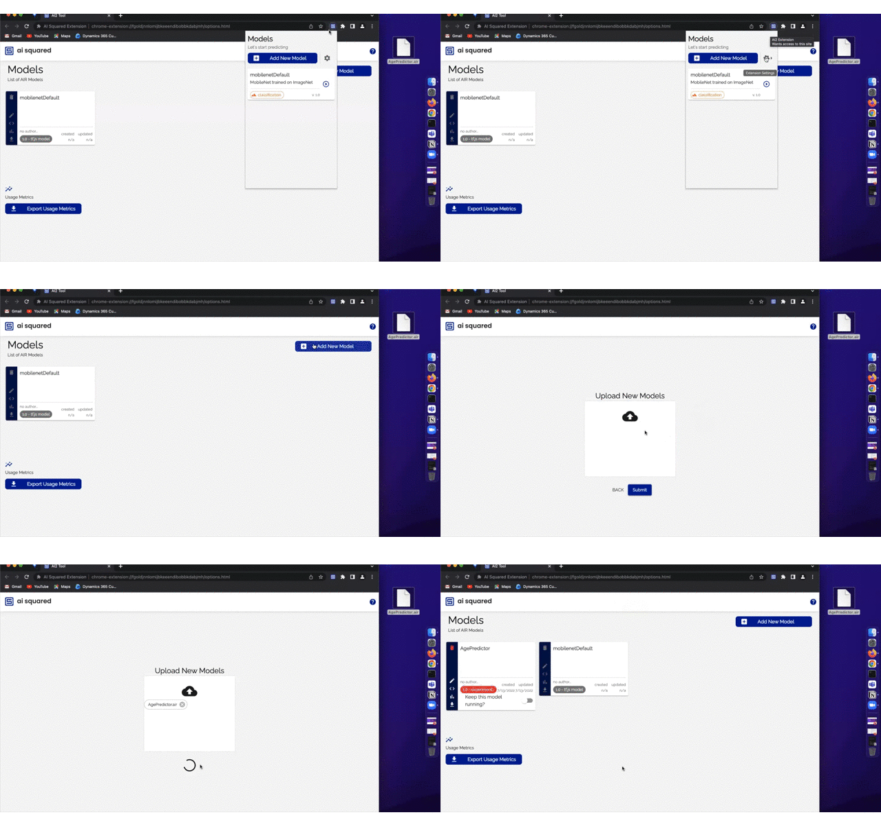
From here, you can load the .air file you made into the browser extension by dragging and dropping it like this:

From here, navigate to a web page that you want to run your model on. Remember that this model was trained on tightly cropped images of faces, so it might struggle with images that deviate too much from its training data. Because of this, we’ll try the model out on a page showing the AI Squared founders.

Now that the .air file is loaded into the extension, it’s ready for use. Clicking on the extension button shows a playlist interface of the models you have available. By clicking on the play button next to the model you want to use, you can see the model results rendering immediately.

Most of these classifications look pretty good, it seems like the model can correctly classify most of these images. Some classifications are definitely off, though…

I know Lloyd is young at heart, but it seems that the model only considered that instead of other clues to his age, like his beard. And I know that being director of Engineering is a stressful job, but it seems the model is really picking up on the toll that is taking with Brian!

Let’s log these instances of misclassification to track the performance of this model. Recall that you created a feedback widget during step 2.6 to simplify logging this information. By clicking this icon that rendered on the screen when you ran your model…

…you’ll get a popup menu with each classification the model made on this webpage. For any or all of the images that were classified you can give binary, thumb up or thumb down feedback.

This feedback is logged to the local database along with additional metadata, and can be downloaded from the extension webapp interface.

After working with this model across multiple web pages, you’ll have a great understanding of the strengths and weaknesses of your model.